Ride the Wave(let) and Get EXCITEd

The motivation of the whole story is a technique called Time-Frequency Analysis, which originates from signal processing. In simple words: it provides the frequency content of a signal (or a simulation result) given as a time trace.
AVL EXCITE™ M is well known and appreciated for its outstanding capability to solve flexible body motion and their mutual contacts (e.g. arising for bearings, gears, pistons) in the time domain. This is a great method to render highly non-linear behavior and maintain full interaction between body motion and contacts. However, NVH-engineers – and humans in general – tend to perceive noise and vibrations in terms of frequencies. Consequently, we need something to convert from time to frequency domain.
Luckily, there is already a rich toolbox available. Let us introduce some useful instruments we have at hand.

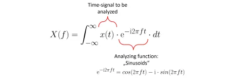
This is the most basic method to move a signal from time x(t) to frequency domain X(f). The idea is simply that you walk along your frequencies f (from  -∞ to +∞ ) and use a "sinusoid" of that frequency as an analyzing function. Multiplying (dot-product) the signal to be analyzed with the "inspecting sinusoid" yields the amplitude and phase angle at a certain frequency. It is actually quite a simple and intuitive process.
For readers addicted to formulas, this can be expressed as shown in Figure 1. For readers disgusted by formulas, simply continue with the mental image of projection onto the analyzing sinusoids.

When looking into this concept a bit more, it becomes obvious that it only works reliably if we have a stationary and periodic signal. Otherwise, the multiplication with the analyzing sinusoids will yield random numbers and the results are simply bullshit. In nicer words: this means that the FT has no ability to render localized frequency content like it emerges from an impact.
But wait! What to do if there is a transient signal to be investigated? Don't panic, stay calm! The answer to this delicate question is in the next paragraph. So, don't stop reading here, you will miss the crucial point!

Before we continue, just a little addition: Fourier Transform functionality and its faster brother, the so called Fast Fourier Transform (FFT), is available to EXCITE M users through AVL IMPRESS™ M and excitePost.

Many of these signals we deal with vary in time, which requires so-called Time-Frequency analysis. The all-time-classic approach used for that is the Short Time Fourier Transform (STFT).
The magic of this method is: A constant window function – similar to a Hann-window used in FT – is applied to a small time section of the signal, where the Fourier Transform is then calculated.
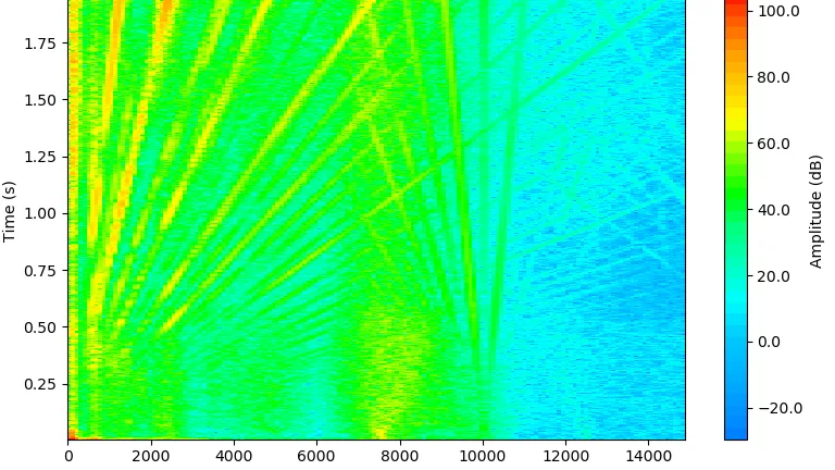
Do this for each time step and put them all together (using a convolution), and you receive a valid Fourier Transform for the non-stationary signal, the plot of which is called a Spectrogram (Figure 2).
(Note that different versions of Spectrograms are common, one with the time-axis on the abscissa one with time-axis as ordinate).

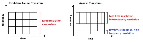
All of this looks good so far, but there is a major shortcoming with the STFT, which comes in the form of a trade-off between time resolution and frequency resolution. This is called the Gabor uncertainty and is analogous to the Heisenberg uncertainty in quantum mechanics. The following Figure 3 provides a visual representation of this uncertainty showing the minimum in the form of an area element of the discretization of the spectrogram, which we will be referring to as "tiling".

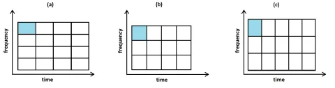
For our spectrogram, this means that we can have high time resolution or high frequency resolution, but not both at the same time. This uncertainty cannot be avoided and is annoying particularly for signals with a very large frequency range.

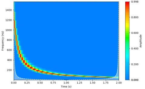
This problem can be seen well in the following example: We will perform an STFT on a hyperbolic chirp signal generated in SciPy. The chirp has the following parameters:

Start: Time t = 0.0 s, Frequency f = 1500 Hz

End: Time t = 2.0 s, Frequency f = 50 Hz

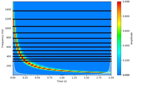
Let's see how well the spectrogram represents these parameters (Figure 4).

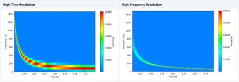
Neither of these spectrograms is optimal for representing our signal. The high time resolution gives a more accurate representation of the hyperbolic chirp towards t = 0 (where f = 1500 Hz), but is visibly "choppy" on the frequency axis, which is especially problematic at the low frequencies.  The high frequency resolution is smoother throughout, but the signal does not even get close to the beginning frequency of 1500 Hz (because the time at which it should reach this frequency is not correctly displayed in the spectrogram!). Even in the left image, the signal doesn't quite reach the 1500 Hz, but if the sampling had been chosen such that it did, the spectrogram would have been completely unreadable on the frequency axis. This poses a significant problem when the frequency range of the signal is large and we would like to read off transients and orders, such as in a motor run-up.

Luckily, there is a way around this in the form of prioritizing the resolution for certain parts of the spectrogram; this is where wavelets enter the stage.

To warm up for the WT deep-dive lets talk about resolution particularities of the WT first.

Typically, low frequency components change slowly over time, so a high time resolution is not required here, but we need high frequency resolution. High frequencies appear for shorter periods of time, meaning that the time resolution plays a role here, but our frequency resolution doesn't need to be as high.

One can see that it makes sense to change the tiling of the spectrogram for the proper resolution in the important areas. The way this is done in the wavelet transform is displayed in the following (Figure 5):

Let's apply the wavelet transform on our hyperbolic chirp from above (Figure 6):

With a linear frequency scale, it is easy to see the tiling, and that we have a representation of our signal that is both accurate to the initial frequency of 1500 Hz and reasonably sampled on the frequency axis.

Having seen the output, you may ask: What does the wavelet transform do? Is it just a fancy STFT window with different tiling? To answer the second question - well, yes, technically speaking. Both methods use a convolution to slide a windowing function across the signal and depend on a time translation and a frequency parameter, resulting in a vector of coefficients representing the magnitudes of the signal at each time, at the given frequency. However, as one moves up the frequency axis (see the tiling), the size of the wavelet is changed. It starts out wide in time and narrow in frequency to catch the smaller frequencies, and gets narrower in time and wider in frequency to look at smaller time increments.

This results a logarithmic “scaling” axis. Note that one should be careful with the word “frequency” axis, as the scaling is not equal but only proportional to the frequency. They must be transformed to frequencies using the sampling time to get useful information from the plot. The plot is called a Scalogram instead of a Spectrogram.

Now Get Ready for the Most Fundamental Point of the WT: The Window-Function

While the tiling is an important aspect of wavelet analysis, our new window functions, the Wavelets themselves, are the most striking aspect.
What does a wavelet look like? Well, pretty much anything, within a few constraints. Figure 7 shows some of the different forms that a wavelet can take:

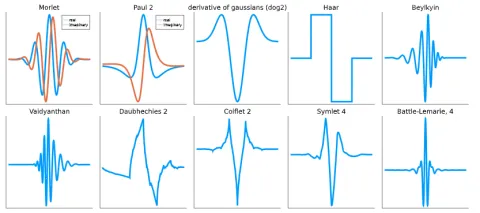
The main property they have in common (besides finite amplitude) is localization, known as a "compact support". This is far from surprising as the alternative, some wave repeating itself over the entire domain, would just result in a normal Fourier Transform.

Other than that, one is free to design a wavelet as desired, with certain mathematical properties being advantageous depending on the wavelet’s purpose.
Looking at the 2nd row of Figure 8 you may think: Ok, but some of the wavelets look more like the scribbling of a toddler. True, but we can assure you that they are well designed and well serve specific needs. For instance, the Daubechies-wavelets play an import role in climate-research because they greatly improve the signal-to-noise ratio of gas-concentration measurements.

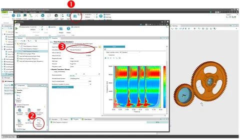
The Wavelet Transform as it is applied in the Time-Frequency-Analysis COMPOSE App. With version 2024 R1 the COMPOSE App Time-Frequency Analysis offers Wavelets in addition to STFT. If can be invoked through the EXCITE M App-Library and is accessible via the main ribbon (Figure 9).

In the Time Frequency Analysis COMPOSE App, the “Morse wavelet” was implemented, which is a so-called “family” as its shape is parameter dependent (Figure 10). This allows for more versatility for the user as the parameter can be shifted for the ideal wavelet shape.

The “ideal wavelet shape” sounds a bit arbitrary, and that is because it is. It primarily depends on two factors: The user’s priority of resolution (time or frequency) and the shape of the signal. Let us start with the more concrete factor: Resolution priority.

Despite the efforts to keep this text light on the mathematical details and theory, the reader may have noticed by now that a significant amount of both flows into performing wavelet analysis. To keep the app as user-friendly as possible, a few truncations are necessary.
The above figure displaying all the possible Morse wavelet shapes, which depend on two parameters, is nice and all, but both these parameters have similar effects on the Scalogram (time/frequency resolution).
So in the COMPOSE App the parameter γ is fixed and only the parameter β  is left up to user input.

Figure 11 shows the effect of the parameter β on an artificial impact signal, which is shown in the logarithmic frequency and magnitude scales to better illustrate the differences.

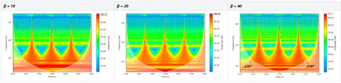
The time/frequency trade-off is clearly visible here. The smaller the parameter β, the higher the time resolution.  The larger β is, the higher the frequency resolution. While the parameter input is in the form of a slider and can be almost continuously varied, the app recommends three values, two of which approximate different well-known wavelets:

• Morlet wavelet: Higher time resolution
• Bump wavelet: Higher frequency resolution

The second factor to bear in mind during choice of the β parameter is the shape of the signal. This is where the more arbitrary portion comes in: A rule of thumb is generally to use a wavelet that has a similar shape to the original signal. With the number of different signals in existence, this is a bit difficult to verify. Thus, it is recommended for the user to try out a few parameters. The answer to the question of whether this is a bonus or a drawback is up to how adventurous the user is.

Besides the wavelets themselves, a feature of wavelet analysis that tends to stick out is the so-called “Cone of influence” (COI) (see Figure 11, right). This is the mysterious character we mentioned in our introduction. It is visible towards the beginning and end of the time axis of the Scalogram. The COI appears due to the difference in signal size and wavelet size, which is not compatible with the convolution. Thus, the signal must be padded with zeros at the beginning and end, causing an interruption in the periodicity in those areas and leading to artifacts. The COI separates the usual area where the artifacts happen from the rest of the signal, and the user should be aware that the area outside the COI should be handled with care.

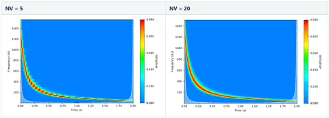
The last input parameter is the “number of voices” (NV), where the user can choose the number of steps between two octaves. A higher number of steps results in a higher frequency resolution (up to the Gabor limit, as we know) at the cost of performance, as there are more coefficients to be calculated along the frequency/scale axis. The difference is visible in the following Figure 12, using our hyperbolic chirp from before.

To further increase your trust in Wavelets we have prepared a real world application example, namely a gear hammering of a single gear stage. While the small gear is driven by a constant speed while the larger gear is exposed to an alternating load torque. This leads to changes in flank contact with repeated impacts, as visible in the time-trace of the gear-connection moment (Figure 13, top).

• Focusing on the time-trace one can identify the following characteristic regions for each of the impacts:
• The actual impact (blue stars) which is so intense that numerous eigenfrequencies of the system get excited
• A phase at which the dominant eigenfrequencies of the system (at about 400 Hz and 800 Hz) decay (1)
• A phase of stationary gear contact with dominating meshing frequency at 2050 Hz (1st) and 4200 Hz (2nd) (2) 

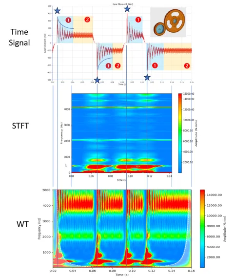
The STFT (Figure 13, mid) is actually not bad but needs quite some tuning to find the best compromise between time and frequency resolution.
However, it eventually manages to resolve the impacts as well as the gear meshing frequencies in a reasonable way.

But now look what the wavelet transform can do! It provides a great picture on what is going on in the system (Figure 13, bottom). The visibility of the local details is simply amazing. One can even see how the gear meshing frequencies get intermitted while the flanks loose their contact. The periodic meshing impacts along the 2050 Hz and 4100 Hz line also gets depicted clearly. Well done, little wavelets!

If you have made it up to this point in the article, you will have realized that the concept of the wavelet transform is nothing mysterious. The opposite is true - it is quite an intuitive method. We hope to have made the term "Wavelet" a bit more familiar to you. It actually uses what the name implies - small waves you translate and scale throughout your signal, thus extracting localized frequency information into a plot called a Scalogram. We have enabled this functionality in the Time Frequency COMPOSE App to facilitate the creation of meaningful plots with more detail than those of the Short Time Fourier Transform. May the wavelet transform be with you and may it serve you well in improving the frequency content analysis of your simulation results.

References and Sources

A great insight into Time-Frequency Analysis is given by Michael X Cohen in his Youtube channel: https://www.youtube.com/playlist?list=PLn0OLiymPak2BYu–bR0ADNBJsC4kuRWs
Here one can find more information about the most intuitive wavelet, the Morlet-wavelet: Morlet wavelet - Wikipedia
Moreover, also MATLAB gives plenty of general information in Time-Frequency Analysis and Continuous Wavelet Transform - MATLAB & Simulink - MathWorks Deutschland
For those looking for more detail on wavelet analysis, we would recommend looking into the book "A wavelet tour of signal processing" by Stéphane Mallat (https://www.sciencedirect.com/book/9780123743701/a-wavelet-tour-of-signal-processing)

Acknowledgement

We want to express our special gratitude to Franz Diwoky, who greatly supervised and supported the development of this feature.