
NVH Analysis of an Electric Water Pump
Published on December 02, 2025 · 2 min read
With the global energy structure transformation and the advancement of the "Dual-Carbon" strategy, the market penetration of new energy vehicles (including pure electric and plug-in hybrid electric vehicles) continues to rise. As a core component of the thermal management system in new energy vehicles, the electric water pump is responsible for cooling the battery, motor, and electronic control system. Its reliability, efficiency, and NVH (Noise, Vibration, and Harshness) performance directly affect the vehicle's safety, energy consumption, and driving comfort.
Unlike traditional internal combustion engine vehicles, electric water pumps in new energy vehicles typically operate at higher speeds and must adapt to frequent start-stop conditions. Their vibration and noise issues are more easily perceived by users in the quiet electric cabin environment, making them a key factor affecting the market competitiveness of high-end vehicle models.
In recent years, consumer demands for vehicle NVH performance have become increasingly stringent, and international standardization organizations (such as ISO) as well as national regulations have gradually tightened limits on in-cabin noise. In this context, the NVH issues of electric water pumps are not only technical challenges but also important breakthroughs for automakers to achieve product differentiation and meet users' high-end demands.
However, NVH optimization of electric water pumps faces the complexity of multi-physics coupling: electromagnetic excitation of the motor, fluid-induced vibration of the impeller, bearing vibration, and structural resonance are intertwined, requiring interdisciplinary collaborative analysis (such as electromagnetic-mechanical-fluid coupling simulation) for accurate root cause identification and effective suppression.

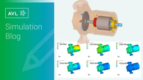
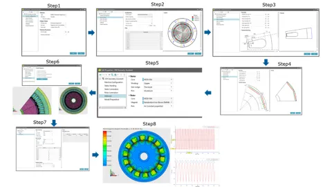
Figure 1 shows a detailed electric water pump model. The detailed NVH evaluation calculation of this electric water pump model is completed by combining electromagnetic simulation, CFD analysis, dynamics simulation, and acoustic simulation methods. The specific analysis process is as follows:
Step 1: AVL E-Motor Tool™
Electromagnetic Simulation → Calculation of Stator Forces and Rotor Torque
Step 2: CFD
3D Computational Fluid Dynamics → Calculation of Flow Characteristics and Pressure Distribution on Structural Components
Step 3: MBD
Multi-Body Dynamics Model → Integration of Excitation Sources from Steps 1 and 2, Considering Impeller and Motor Rotor Dynamics (Including Sliding Bearing Characteristics)
Step 4: EAC
Aerodynamic Noise Calculation → Acoustic Simulation via EXCITE Acoustics

As a professional electromagnetic simulation software in the AVL software platform, the AVL E-Motor Tool™ (EMT) can conveniently and quickly perform motor-related electromagnetic field simulations, providing accurate load boundaries for subsequent motor performance matching, 3D thermal management, and motor dynamics analysis, enabling seamless interaction of electrification simulation data within the AVL platform.
Based on the Geometry Assistant module in the EMT, users can define the motor cross-sectional model through geometric input or imported CAD, while also performing material property assignment and meshing. Combined with the Model Assistant module, electromagnetic field calculations for the motor under different speed and torque conditions can be achieved. The entire process is convenient and efficient.
The current model motor has 7 pole pairs, 42 stator teeth, and is structured as a PMSM distributed single layer. The electromagnetic calculation results of the motor are shown in figure 3 below.
AVL FIRE™ M, as a professional CFD simulation software, includes the Embedded Body immersed boundary method, which enables fast and accurate simulation of general flow fields. This method does not require meshing of moving parts. Instead, the entire solution domain is meshed (background mesh), and then the computational boundaries are embedded into the background mesh. The fluid-solid interface is identified through numerical methods, making it suitable for complex computational boundaries or scenarios with moving boundaries.
To accurately consider the flow around embedded objects, the Embedded Body method extends the discretization capability of the Navier-Stokes equations, focusing on gradient calculation and boundary condition handling at the fluid-solid interface. In this case, based on this method, both the fluid and solid domains are considered without the need to mesh the water pump rotor, enabling rapid calculation of the loads on the rotor and housing walls.
The model boundaries are as follows: water pump inlet flow rate is 4.75 m³/h, water temperature is 25°C, pump speed is 3500 rpm, and outlet pressure is 10 bar. The boundary definitions are shown in figure 4 below.

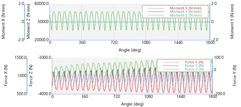
Based on the CFD calculation of the water pump blade pressure data, combined with the calculation method shown in the figure below, the blade rotor torque and forces are equivalently converted using a custom Formula in the software.

The converted rotor torque and forces are shown in the figure below.
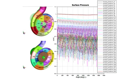
Different areas are defined on the housing surface to map and output the transient pressure at different locations. The specific area division and pressure amplitudes in different areas are as follows:
Finite Element Model Setup
The dynamics model of the electric water pump is built based on AVL EXCITE™ M. The main geometries in the model include the water pump housing and rotor. The rotor mesh and reduced model are shown in the figure below. The specific main nodes of the reduced model include the water pump blade load application point, front sliding bearing elastohydrodynamic (EHD) connection point, bearing connection point, and motor center point. The modes of the reduced .exb file meet the analysis requirements.
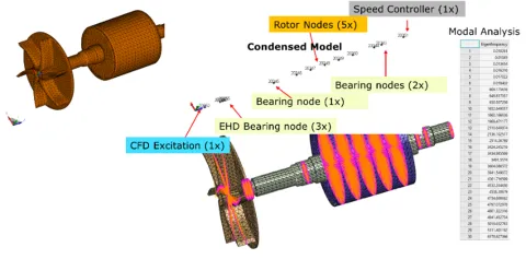
The entire water pump housing is a linearized model. The specific main nodes of the reduced model include the water pump pressure load application surface, front sliding bearing EHD connection point, bearing connection point, and motor stator connection point. The modes of the reduced .exb file also meet the analysis requirements. Since pressure boundaries need to be applied in the dynamics model later, a substructure load step must be added during the model reduction process, as shown in the figure below:


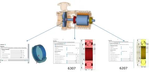
Joint Definition
The key joints in this dynamics model include the front sliding bearing EHD joint and the roller bearing joints at both ends of the motor. Based on the powerful sliding bearing analysis module in EXCITE M, not only can sliding bearing support be accurately considered, but potential wear risks of the sliding bearing can also be evaluated.
Load Application
The load boundaries in the model include the water pump rotor radial force, axial force, and torque; housing water pump wall pressure; and motor electromagnetic excitation. The specific load application is as follows:
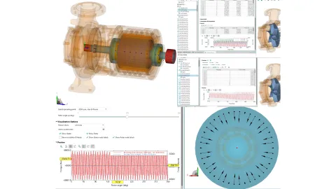
Dynamics Results
The simulation corresponds to speeds from 1000 rpm to 3500 rpm. The simulation results show stability at all speeds. The bearing forces are relatively reasonable, and no bearing knocking occurs during operation.
The maximum rough contact pressure of the front bearing is close to 75 MPa. The rough contact pressure distribution of the bearing indicates a risk of partial wear at the front end of the bearing.

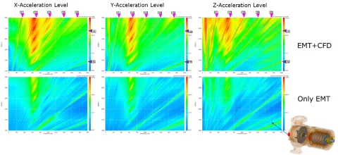
The figure below shows the XYZ three-direction vibration acceleration results at the nodes of interest on the motor housing and water pump housing surface. Since the front water pump rotor has 6 blades, there is a 6th-order harmonic component in the liquid pressure during operation, resulting in larger vibration amplitudes at the 6th, 12th, 18th, 24th, and 30th orders on the housing surface. At the same time, the application of motor electromagnetic excitation also leads to larger vibration harmonic amplitudes at the 42nd and 84th orders of the motor.

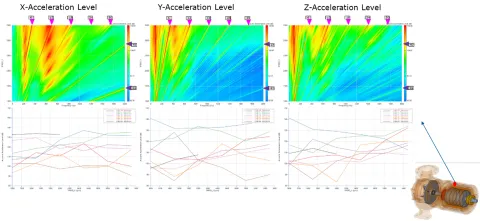
Combined with the vibration results on the electric water pump housing surface, there is a significant resonance band between 600–700 Hz. Based on the modal analysis of the water pump system, obvious housing system modes are present near 636 Hz and 648 Hz. Targeted optimization can be performed in subsequent structural improvements.
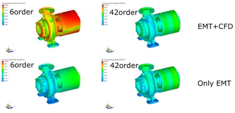
The figure below shows the vibration contours of different main orders of the electric water pump at 3500 rpm. Overall, the vibration amplitude of the water pump housing is larger than that of the motor housing.

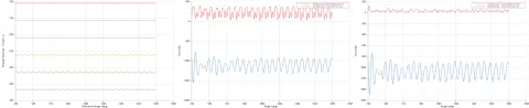
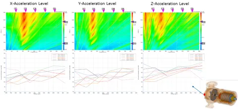
The figure below shows a comparison of results after removing the water pump excitation. Visually, after removing the water pump excitation, the vibration amplitude on the water pump housing surface is significantly smaller than when all excitations are considered.
The vibration contours on the housing surface show significant changes in the amplitude of the main orders of the water pump excitation. The housing vibration increases significantly when the water pump load excitation is applied, while the vibration changes on the housing surface for the high-frequency main orders of the motor are relatively small.
EXCITE Acoustic, based on the WBT meshless algorithm, quickly calculates the radiated sound field of the housing by defining the vibration boundaries on the housing surface.
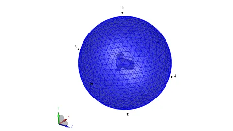
The figure below shows the sound pressure level for six microphones and the radiated sound field contours. The highest sound pressure level for different microphones is close to 70 dB. The sound pressure level is higher at the 6th order.

By combining the AVL simulation platform, electromagnetic load calculation of the electric water pump, water pump flow field analysis, subsystem dynamics simulation, and radiated sound field analysis can be achieved. This provides a full-process simulation toolchain for the NVH simulation of electric water pumps.
Stay tuned
Don't miss the Simulation blog series. Sign up today and stay informed!
Read More About This Topic

NVH calculations provide information about resonant speeds and frequencies, but the cause of resonances themselves cannot be easily determined. In order to find root causes of faults or problems, Root Cause Analysis should be carried out.
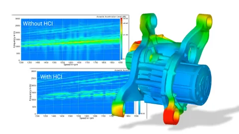
As electric vehicles enter the mainstream, NVH (Noise, Vibration, Harshness) has become a top quality criterion. A promising solution is Harmonic Current Injection (HCI), which can now be simulated virtually to tackle NVH issues before the first prototype exists.
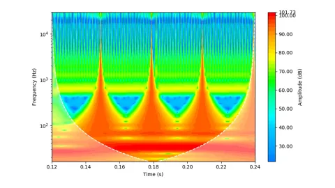
This article is about a technique called Time-Frequency Analysis, which originates from signal processing. In simple words: it provides the frequency content of a signal (or a simulation result) given as a time trace.
The fourth part of this online event series focuses on AVL's simulation solution for electric drive development. Learn about the opportunities that virtualizing can provide. Especially when it comes to using a consistent set of simulation tools for a streamlined workflow.
Stay tuned for the Simulation Blog
Don't miss the Simulation blog series. Sign up today and stay informed!