


Dynamic Roughness Adjustment for Optimizing Main Bearing Designs with AVL EXCITE™ M
Published on October 15, 2025 · 9 min read

Designing crankshaft main bearings in combustion engines is a complex engineering challenge. These components must withstand high loads and ensure long service life under varying operating conditions. Traditional simulation methods – especially multi-body simulations with flexible bodies – have proven effective in modeling the interaction between structure, lubricant, and load.
However, the introduction of surface texturing for performance optimization has added complexity. Under high hydrodynamic and asperity contact pressures, these textures wear off, altering the bearing surface and its load-carrying behavior. This necessitates a more dynamic and precise simulation approach.
This study introduces a new simulation method in the 2025 R1 release of AVL EXCITE™ M that dynamically adjusts surface roughness based on wear depth during operation. Unlike previous models that use fixed or periodically updated roughness values, this approach continuously updates roughness parameters throughout the simulation.
This dynamic modeling allows for a more realistic representation of the wear process and better alignment with real-world operating conditions.
The simulation is based on an elasto-hydrodynamic (EHD) model integrated into a detailed multi-body simulation using EXCITE M. Key features include:
- A flexible engine housing and a rigid crankshaft section.
- Real measured surface profiles used to define initial roughness.
- Iterative wear simulation: after each step, both the bearing contour and surface roughness are updated.
- A wear depth limit of 0.1 µm per iteration and a total simulated runtime of 5000 hours.

To accurately simulate wear behavior in main bearings, the study integrates real-world surface measurements into the simulation model. This approach ensures that the simulation reflects the actual conditions experienced by engine components during long-term operation.
Real Surface Profiles
Surface roughness data was collected from bearings subjected to real endurance testing. These surfaces were analyzed using white light interferometry, a high-resolution optical method that captures 3D surface topography. The resulting data was processed using the Micro-Contact Analysis tool, which extracts key roughness parameters such as:
- Summit Roughness (RMS): Standard deviation of peak heights.
- Mean Summit Height: Average height of surface peaks above the mean line.
These parameters are essential for modeling solid contacts using the Greenwood & Tripp theory.
Wear-Dependent Roughness Evolution
To simulate the progressive smoothing of the bearing surface due to wear (also known as "running-in"), the model dynamically adjusts roughness values based on local wear depth. This is achieved through:
- A lookup table that maps wear depth to roughness values.
- Linear interpolation between measured states (e.g., 0 µm, 1 µm, and 15 µm wear depths).
- Separate treatment of the upper and lower bearing shells, with the lower shell experiencing more wear due to load distribution.

These values show a clear trend of surface smoothing with increasing wear, particularly in the early stages where high asperities are quickly worn down.

To evaluate the effectiveness of the dynamic roughness approach, the study compared two simulation variants under identical operating conditions:
- Variant A: Surface roughness remains constant throughout the simulation.
- Variant B: Surface roughness is dynamically updated based on local wear depth.
Test Conditions
Both simulations were run for 5000 hours of operation at a critical operating point:
- Engine speed: 1500 rpm
- Load: High (representing full-load conditions)
This scenario was chosen because it represents a worst-case condition for wear, with frequent solid contact due to thin lubrication films.
Wear Depth Comparison

Variant B exhibited 46% less wear than Variant A, highlighting the significant benefit of modeling surface evolution.
Surface Roughness Evolution
In Variant B, the dynamic model captured the smoothing effect of wear, where high asperities are worn down early in the bearing’s life. This led to:
- Reduced contact pressure
- Delayed onset of solid contact
- Lower cumulative wear


One of the most insightful visualizations in the study is Figure 5, which shows the distribution of surface roughness values across the bearing shell after 5000 hours of simulated operation using the dynamic roughness model (Variant B).
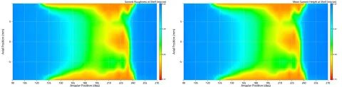
Figure 4 illustrates how wear is not uniformly distributed across the bearing surface and in Figure 5 we can make the following observations:
- Edge zones show higher smoothing due to increased structural deformation and localized contact.
- Central zones retain slightly higher roughness, indicating less intense contact pressure.
The roughness values at the most worn location were:
- Summit Roughness: 0.168 µm
- Mean Summit Height: 0.182 µm
This represents a ~68% reduction from the initial roughness, confirming the effectiveness of the dynamic model in capturing the running-in effect.
Engineering Implication
Understanding the spatial distribution of roughness is crucial for:
- Designing oil grooves and supply channels to match wear patterns.
- Targeting surface treatments (e.g., coatings or texturing) where they are most needed.
- Improving predictive maintenance by identifying zones of accelerated wear.
This figure reinforces the value of localized modeling in tribological simulations and supports the case for using real surface data in predictive wear analysis.
One of the most critical findings of the study is visualized in Figure 6, which compares the contact pressure as a function of lubrication gap height for two surface conditions:
- Initial (unworn) surface
- Worn surface after 5000 hours

Why This Matters
The Greenwood & Tripp model is highly sensitive to surface roughness parameters. As the surface wears and becomes smoother (due to the removal of asperities), the contact pressure curve shifts:
- Initial surface: Contact pressure rises earlier with increasing proximity, indicating more frequent solid contact.
- Worn surface: Contact pressure rises later, but more steeply, indicating less frequent but sharper contact events.
This shift has two major implications:
- Reduced Wear Rate: Smoother surfaces reduce the frequency and intensity of solid contact, leading to lower wear over time.
- Improved Predictive Accuracy: By dynamically updating surface roughness in the simulation, the model better reflects real-world behavior, especially under mixed lubrication conditions.
This figure underlines the importance of modeling surface evolution in tribological simulations. It validates the core innovation of the study: that dynamic roughness modeling significantly enhances the reliability of wear predictions.
This study demonstrates that dynamically modeling surface roughness during wear simulation significantly improves the accuracy of wear predictions and bearing life assessments.
The method:
- Reduces overestimation of wear.
- Reflects real-world surface smoothing effects.
- Enhances the reliability of simulation-based bearing design.
- This approach represents a valuable advancement in tribological simulation and offers OEMs and bearing manufacturers a powerful tool for future development.
Stay tuned
Don't miss the Simulation blog series. Sign up today and stay informed!
Read More About This Topic

We are proud to present our latest software release 2025 R1.
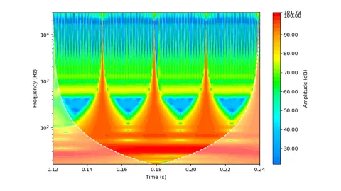
This article is about a technique called Time-Frequency Analysis, which originates from signal processing. In simple words: it provides the frequency content of a signal (or a simulation result) given as a time trace.

When designing gears, engineers generally rely on existing industry standards. However, these standards can only consider what is currently known. Innovative designs that go beyond that require research.

NVH analysis is typically performed after a problem has been identified that needs to be addressed. In the case of a simulation model used, it is advisable to proactively look for increased vibration and resonance so that the model can be optimized before the first prototype is built.
Stay tuned for the Simulation Blog
Don't miss the Simulation blog series. Sign up today and stay informed!