
Master Debugging in AVL EXCITE™ M Step by Step
Published on April 07, 2026 · 10 min read

In practice, debugging often feels slower than we would like. Errors interrupt the workflow, convergence issues raise questions, and unexpected results challenge our assumptions. But this phase is not a sign of failure - it’s where models mature from an initial setup into a representation you can trust. Across many projects, we see the same underlying challenges appear again and again. Input data may be incomplete or inconsistent. Boundary conditions might unintentionally contradict physical assumptions. Numerical stability issues can arise during transient events. Sometimes the simulation runs - but the results simply don’t look right at first glance.

If this sounds familiar, you’re not alone. These situations are a normal part of building advanced models, and they occur even in well-designed setups. What matters is how quickly and systematically you can move from “something’s wrong” to “I understand what’s happening.”
The goal of this article is to help you do exactly that - by sharing practical debugging strategies and highlighting how AVL EXCITE™ M is designed to support you during this critical phase. With the right approach, debugging becomes less about being stuck - and more about progressing confidently toward meaningful simulations.
Unexpected results rarely resolve by rerunning the same simulation. Progress comes from narrowing down possible causes in a structured way - from broad checks to targeted changes.
Check the Basics
Confirm units, parameter ranges, and initial conditions. Small inconsistencies here can strongly influence results and obscure the real cause.
- Tip: Before changing advanced settings, double‑check units, orders of magnitude, and initial conditions. Small inconsistencies here often cascade into larger problems later.
Simplify the Model
Temporarily reduce the model to its essential components. Removing non-critical elements often makes the source of unexpected behavior clearer.
- Tip: Switching flexible bodies to rigid can sometimes simplify complex modeling problems and make the source of instability easier to isolate.
- Tip: Temporarily disable optional joint features, like friction, damping add‑ons, or secondary force components. Reducing these effects often removes numerical complexity and makes it easier to pinpoint where instability or unexpected motion originates.
- Tip: When a joint primarily serves to prevent motion in a direction where no significant forces act (e.g., an AXBE stiffening a shaft), try removing that degree of freedom from the body rather than adding a joint. This reduces constraint complexity and often improves stability.
Review Diagnostics
Warnings and log messages provide valuable clues. Early or repeated messages often indicate where assumptions or numerical limits are being challenged.
- Tip: Store results for each time step, especially the steps immediately before the issue appears. Reviewing these fine‑grained results can help pinpoint where the problem first emerges.
Change One Thing at a Time
Adjust one parameter at a time and observe the effect. This makes it easier to understand what influences the outcome and builds confidence in the final setup.
- Tip: During debugging, reduce the simulation interval to the shortest time span that still reproduces the issue. Faster runs allow quicker iterations and make it easier to analyze diagnostics around the critical event.

Together, these techniques help turn debugging from a source of delay into a structured process. Instead of repeatedly asking “Why doesn’t this work?”, the question becomes “What does this tell me about my model?” - a much more productive starting point.
Effective debugging relies on understanding what changed, where complexity matters, and why the solver reacts the way it does. EXCITE M provides tools that support this way of working by making changes, structure, and feedback visible.
Understanding What Changed
Many debugging issues emerge after incremental model updates - a new component, a parameter adjustment, or an updated dataset. UI‑based differencing and file‑level input comparisons allow users to quickly identify what has actually changed between model versions, without relying on memory or manual checks.
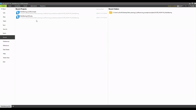
This makes it easier to follow the “change one thing at a time” principle and prevents unrelated modifications from obscuring the true cause of an issue.
Reducing Complexity Without Losing Structure
As models grow, understanding their behavior becomes increasingly difficult - not because the physics are wrong, but because too much is happening at once. EXCITE M’s layering concept supports a structured way to reduce complexity without dismantling the model itself.
By grouping functional parts of a model into layers, specific subsystems can be temporarily switched off to focus on a smaller, more manageable portion of the overall system. This makes it easier to isolate the source of unexpected behavior while maintaining the original model structure.
Reduced models also simulate faster, which supports quick iteration during debugging.
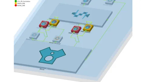
Once the behavior of an isolated section is understood, additional layers can be reactivated step by step, allowing complexity to be reintroduced in a controlled way.
Layers are equally valuable during visualization. In large 3D scenes, temporarily hiding non‑relevant groups helps direct attention to the area under investigation - reducing visual clutter and making physical interpretation more intuitive during debugging.
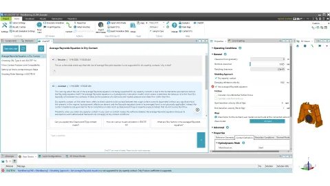
Using Diagnostics as Guidance
Error messages, warnings, and logs in EXCITE M are designed to provide context about solver limits, physical assumptions, and numerical behavior. These diagnostics help narrow attention to the locations where assumptions may no longer hold - often long before a simulation fails completely.
Interpreting these messages early can significantly shorten the debugging cycle, especially when combined with simplified test cases.
When questions remain, EXCITE M’s integrated chat‑based assistance (ChatSDT) helps users articulate problems more precisely - and enables faster, more effective collaboration with support when needed.
ChatSDT was first released in 2024 R2 and integrated into the EXCITE M GUI in 2025 R1. You can refer to this blog article for a more detailed overview and use cases: ChatSDT in Release 2025 R2.
Every successful simulation model goes through a phase where assumptions are tested, limits are reached, and unexpected behavior needs to be understood. Debugging is not a distraction from simulation work - it’s the step that turns a model into a tool you can trust.
By approaching debugging systematically - checking fundamentals, simplifying where needed, using diagnostics deliberately, and making changes incrementally - many issues can be clarified quickly and confidently. EXCITE M is designed to support this way of working, helping you focus on understanding the model rather than fighting it.
Ultimately, the goal isn’t to eliminate debugging, but to make it predictable, manageable, and productive - so you can spend less time stuck, and more time simulating.
Stay tuned
Don't miss the Simulation blog series. Sign up today and stay informed!
Read More About This Topic
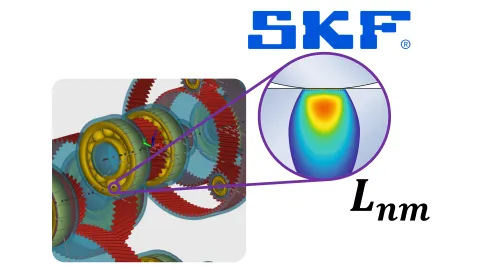
Use the SKF online calculation service directly within AVL EXCITE™ M to evaluate rolling bearing lifetime accurately and seamlessly in your simulation workflow—based on ISO 281, SKF Rating Life, and the SKF Generalized Bearing Life Model.
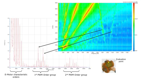
Discover how electromagnetic excitation integrated in multi-body dynamic simulation enable high-fidelity NVH analysis for electric motors with AVL EXCITE™ M.

NVH analysis is typically performed after a problem has been identified that needs to be addressed. In the case of a simulation model used, it is advisable to proactively look for increased vibration and resonance so that the model can be optimized before the first prototype is built.

As electric vehicles enter the mainstream, NVH (Noise, Vibration, Harshness) has become a top quality criterion. A promising solution is Harmonic Current Injection (HCI), which can now be simulated virtually to tackle NVH issues before the first prototype exists.
Stay tuned for the Simulation Blog
Don't miss the Simulation blog series. Sign up today and stay informed!