AVL Simulation Software Release 2024 R1
Published on May 02, 2024 · 39 min read

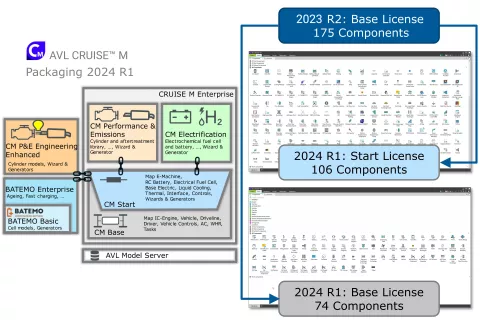
Start and Base Licenses – Application-Focused Packages
AVL CRUISE™ M offers over 300 components, classified into a base license package expanded by addon license groups that deal with advanced functionalities in the electrification and engine performance areas. To offer more application-focused component libraries, this version of CRUISE M splits the licensing of around 260 base components. A newly introduced licensing group "Start" holds around 170 components from the electrification, gas path, cooling, thermal and controls domains. The remaining 90 components in the base package comprise the refrigerant, mechanical, and vehicle domains, including dedicated vehicle control functionalities. The new license group allows you to tailor the component and licensing scope more precisely to the needs of your application.
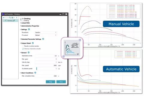
Climbing Performance
The climbing performance of a vehicle is a metric that expresses the maximum possible road gradient a vehicle can climb at a given velocity and gear. Simulating this characteristic helps to tailor the design of the involved torque sources, the drivetrain, and the vehicle itself. To facilitate this specific type of simulation task, CRUISE M offers a new climbing component that bundles all required inputs. In the results, you will find time-based data offering insight into the calculation approach and data for climbing force diagrams, showing the maximum possible inclinations over vehicle velocity for each gear. Climbing performance simulations in CRUISE M are not restricted to certain basic powertrain configurations, and can be run out of the box, for BEV or HEV layouts.
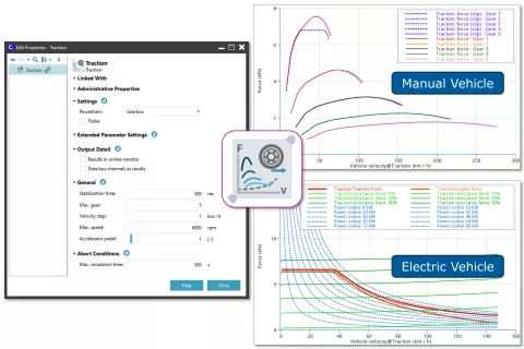
Traction Force
The traction force of a vehicle is the force transferred from the driven wheels to the road. It depends on the characteristics of the torque sources, drivetrain losses, transmission ratios and specifics of the vehicle itself. To shorten the setup of such simulations, CRUISE M offers a new traction component that bundles all required inputs and takes care of running the task. In the results, you will find a new traction folder that holds data on iso-power lines, the traction resistance for different road inclinations, traction force and surplus force (i.e. traction force reduced by the resistance force) calculated for different gears. Traction force simulations in CRUISE M are not restricted to certain basic powertrain configurations; they can be run, out of the box, for BEV or HEV layouts.
ph-Diagram on Circuit Level – Interactive Alignment of Initial Conditions
The ph-diagram of a refrigerant circuit is one of the most compact and explanatory summaries of the components' operating conditions and the overall system performance. CRUISE M provides ph-diagrams online during a running simulation and as part of its postprocessing. Recognizing that unfavorable initial conditions cause additional computational efforts, there is a need for a possibility to align different component initial conditions on the system level. This version of CRUISE M addresses this need with interactive ph-diagrams on the circuit level. If you would like to modify one or the other initial value, you can simply move any operating node to a position that fits your needs.
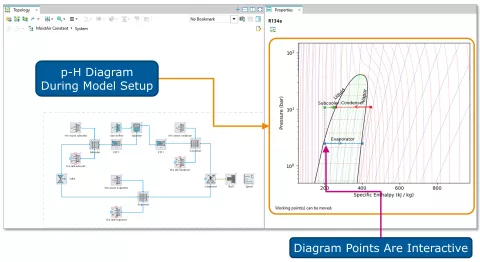
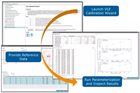
Plate Heat Exchanger Parameterization Wizard
CRUISE M offers a tailored plate heat exchanger (PHE) component that allows for detailed parameterization of geometry, pressure drop and heat transfer. To support this demanding work, a dedicated parameterization wizard is released with this version of CRUISE M. To begin, you only need basic geometric information about your PHE and reference data from measurements or other sources that characterize its behavior under different operating conditions. Next, on the second page, you can select which model parameters (i.e. physical phenomenon) you want to optimize. After that, you can launch the actual parameterization process. Upon clicking the "Finish" button, all parameters are automatically transferred to the genuine plate heat exchanger component, which is then ready to be used in any kind of a refrigerant circuit.
Refrigerant Circuit – Increased Speed and Robustness
The numerical robustness and computational demands of refrigerant circuits exceed those in other physical domains. Modern refrigerant systems feature complex networks that combine different heat sources and sinks (e.g. passenger cabin, battery, e-motor, radiator) that may be alternately operated in heating or cooling modes or put on idle. The refrigerant medium itself is meant to change its aggregate state, causing density variations of three orders of magnitude. This version of CRUISE M addresses the need to computationally simulate such systems effectively, close to real-time. The application of analytical methods to assess system gradients is invoked into the existing numerical solution procedure. Performance measurements reveal speedups between 10 % and 40 %, depending on the model size, while maintaining identical results.
AVL CRUISE™ M New Pre-Chamber Component for Reciprocating and Rotary Piston Engines
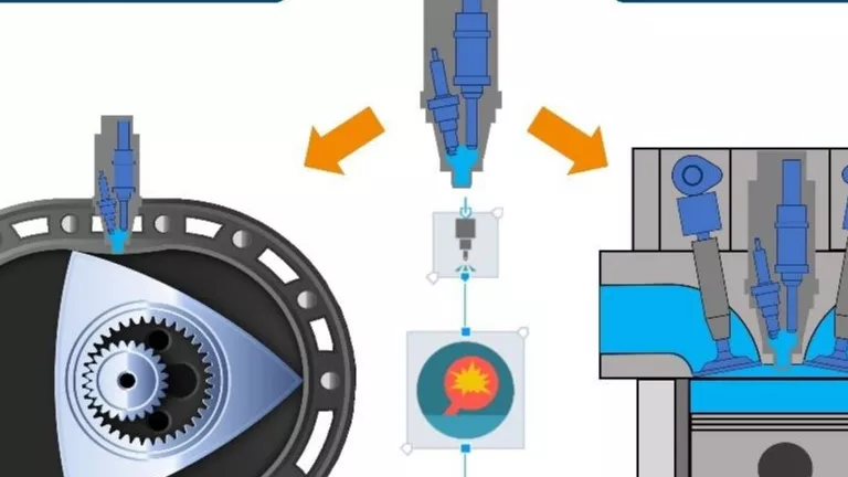
Pre-chambers are commonly used to improve the combustion efficiency of spark-ignited engines. AVL CRUISE™ M 2024 R1 takes this into account with a new pre-chamber component.
The new component offers all explicit combustion models (i.e. table, vibe, two-zone multi-vibe), pollutant formation and wall heat loss models as known from the standard Combustion Chamber component. Setting up models featuring pre-chambers is straightforward. A Cylinder Block component is pulled from the library and the option for direct or indirect injection with Pre-chamber is selected. CRUISE M then automatically creates the correct component assembly with the combustion chamber, valves, injectors, pre-chamber, and prechamber orifice(s). The layout can then be adapted interactively as required. The inclusion of multiple pre-chambers is also possible.
The new Pre-Chamber component can be applied to both reciprocating engines and rotary piston engines.
A dedicated installation example demonstrates how to set up a pre-chamber that is alternately connected to three different combustion chambers of a rotary piston engine depending on their angular position.
AVL CRUISE™ M Extensions of Engineering Enhanced Cylinders & Wizards
With v2024 R1 the Engineering Enhanced Cylinder components and Wizards for gasoline and diesel engines have been enhanced with several functionalities.
The Engineering Enhanced Diesel Cylinder now
- offers a more detailed insight into the wall heat loss distribution to the liner, piston and deck. The data can be monitored by connecting to the corresponding data bus channels.
- allows to parameterize the maps of hydraulic injection delays as a function of "Fuel mass per cycle", "Timing" and "Energizing time".
- enables parameterization of the maps of "Post n injection: CO to THC ratio correction" (n = 1,2,3) given on the manual emission refinement page, as a function of "Fuel per cycle post injection" and "Timing post injection".
- provides a new option to compensate for pressure waves during the active calculation of the Fuel Injection Equipment (FIE) quantity. It can be activated via a check box.
The Engineering Enhanced Diesel Cylinder now
- allows to smooth the output of the exhaust temperature after a fuel cut with a PT1 filter.
AVL CRUISE™ M Aftertreatment Modelling Enhancements
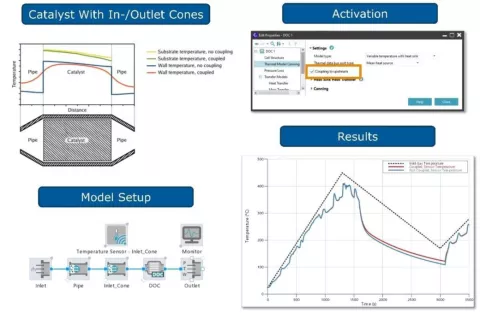
Thermal Wall Coupling: The temperature given at the tip of a thermocouple is a result of convective heat transfer from the exhaust gas and conductive heat exchange with the wall. Under non-flow, soak conditions, the latter effect is dominant This version of CRUISE M addresses this requirement and raises the accuracy of its wall temperature model by introducing a thermal wall coupling of adjacent aftertreatment components.
E-Heater: A new component E-Heater is made available to allow modelling the impact of electric heating of aftertreatment components on their species conversion performance.
Aftertreatment Doser: With this version of CRUISE M, the input dialogs of the Aftertreatment Doser component have been modified to couple the specification of the injectable fluids with those that have been defined on the level of the corresponding gas circuit.
Catalyst and Particulate Filter: For the Catalyst and Particulate Filter components, new data bus channels have been introduced.
AVL EXCITE™ M
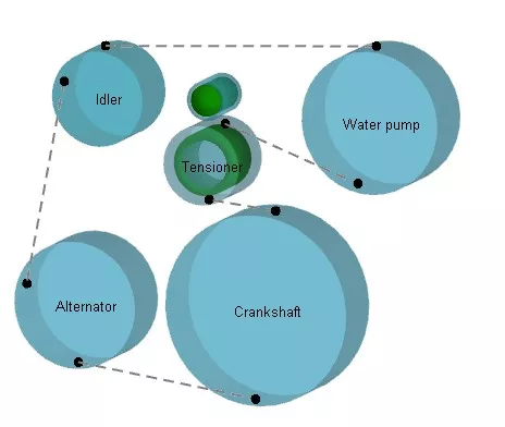
Simple Belt Connection in AVL EXCITE™
Belt drives are key elements in ICEs and hybrid powertrains. The belt joint that was available in AVL EXCITE™ Power Unit is now integrated in AVL EXCITE™ M. The belt is defined inside the macro that provides direct pulley selection, 3D visualization and animation. It also centralizes the definition of belt properties and supports the specification of stiffness and damping, based on specific values.
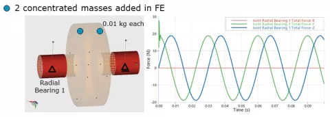
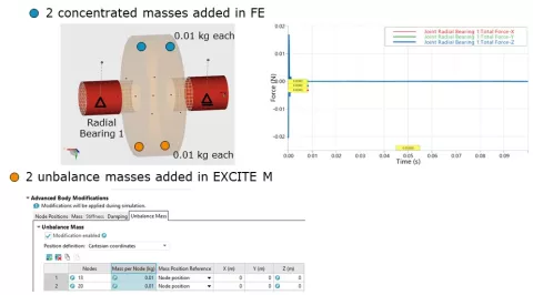
Automated Shaft (Un-)Balancing
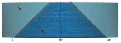
Condensing FE bodies, like crankshafts or electric motor rotors, using third-party FE tools for optimization workflows where the geometry and mass are changing can be computationally expensive and time consuming. This new feature streamlines structural matrix adaptations directly within the EXCITE M solver, eliminating the need for repeating condensation for adding (un-)balance mass. The following figures demonstrate the balancing of an initially imbalanced shaft with a disc, achieved through the precise placement of unbalance masses in EXCITE M.
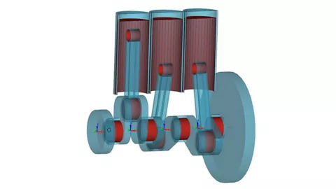
Combine Piston Assembly to One Concentrated Mass
Crank train models in EXCITE Power Unit often represent the piston and piston pin masses through one concentrated mass rather than treating them as separate bodies. Now a concentrated mass option is also available in the ICE assembly of EXCITE M.
Extensions for AXHD Contact Orientations
Until now, in the Advanced Axial Slider Bearings (AXHD), the contact direction and orientation of the subcomponents thrust plate and frustum were coupled. This required a manual rotation of the components to establish a contact direction in the negative direction. Now, the contact direction is decoupled and can be adjusted directly, without having to rotate the components.

For frustums, the contact direction is now automatically set based on the geometry. No rotation is necessary to establish a proper connection.
Wear Analysis App for HD Joints
A new Wear Analysis App has been introduced in the EXCITE M app library. It enables a set up of a wear workflow for the HD joint group (Advanced Radial Slider Bearing, Advanced Sliding Guide and Advanced Axial Slider Bearing). The main benefits of this workflow for wear analysis are automated parameter setting, case definition, job submission and updating surface wear profiles according to the results of previous cases.
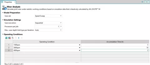
Wear Analysis Workflow – Maximum Wear Depth Limit
Three options are available for the maximum wear depth:
- Auto – Maximum wear depth per iteration calculated automatically so that the wear depth simulated in that iteration does not exceed the composite summit roughness values.
- None – Each selected case is simulated in a single simulation iteration and the wear depth results will be scaled with the appropriate accumulation time.
- User Defined – manually set a maximum wear depth value.
Wear Analysis Workflow – Case Execution
Two options are available for case execution: parallel and sequential. Sequential case execution allows you to specify the order in which the cases should be run, simulating real-life operating conditions, perhaps on a test bed or in the field. The resulting wear profiles of the previous case are used as the input for the next case. Parallel case execution is the quickest option as the cases are submitted in parallel and wear profiles are calculated using a percentage of the operation time requested. At the end of each parallel run, the wear profiles of each body are summed up to be used as the input for the next parallel run of cases.
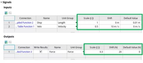
Full Support for Signal Properties
Many components in EXCITE M, such as sensor, function or interface components but also some joints, have a signal section showing specific properties of each input and output signal. Previously, these settings were supported only partly for some of the components. With this release, the scale, shift and default value properties are now fully supported by all components, which improves the overall signal network in EXCITE M.
MFC-Based Model for the EESM
Magnetic field Computation (MFC)-based models are introduced for the Electrically Excited Synchronous Motor (EESM). They are based on magnetostatic simulations over the complete stator and excitation current range or a subset that are imported with the EMC Model Assistant available in the app library. The MFC-based model parameters are evaluated and stored in an e-motor file. Alternatively, linear and saturated fundamental wave models can be parameterized.
The parameter space of the MFC-based model is four-dimensional and covers the rotor angular position, two transformed stator currents and the excitation currents. Due to the relatively high amount of data, rotor eccentricity is not considered.
Enhanced Time-Frequency Analysis AVL COMPOSE™
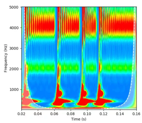
For a better representation of the signal content, high time resolution for high frequencies and low time resolution for low frequencies are required. This property can be accomplished by the Wavelet Transform (WT), which uses a more abstract window function (mathematically a convolution kernel) that changes its location in time (translation) but also its temporal extension (scaling). This results in a so-called scalogram, allowing for the desired varying time-frequency resolution. The increased localization of distinct frequencies, such as system eigenfrequencies and excitation orders, provides a clearer graphical representation of simulation quantities.
The illustration shows a scalogram of the structural response from a run-up simulation of an Electric Drive Unit (EDU). The evolution of the orders imposed by the electric motor and their local amplification by the system's eigenfrequencies are rendered in high detail. The implementation of the WT also highlights regions ("Cone of Influence", COI) which are potentially affected by the particularities of the applied method and should therefore be excluded from the result assessment (indicated by dashed white lines in the right and left lower corners).
AVL EXCITE™ Power Unit
Export to AVL EXCITE™ M Extensions
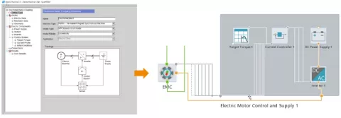
Moving models with EMC joints to the EXCITE M is now easily possible. All configurations and parameters, including those for the electric motor control and supply assembly, are seamlessly transferred.
E-Motor Tool Support for Skewing of PMSMs
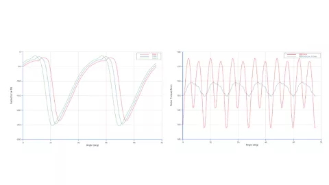
Previously, only models based on the Magnet Force Coupling (MFC) method included a detailed simulation of skewing in EXCITE M simulations. Now, all PMSM models can handle different types of skewing: linear, V-shaped or arbitrary skewing. You can easily define the length of each section and its offset from the standard mechanical angle.
Saturated (2D) fundamental wave models and map-based (efficiency) models require minimal additional simulation effort, as the multi-slice approach is evaluated from the available maps. Linear fundamental wave models and map-based (torque/tooth force) models automatically set up the required slices and evaluate the summed machine parameters.
Significantly reducing project turnaround times and accurate physical models are the main focus of the innovations in this release. Find out about the highlights of the latest release in our battery solution area.
Electrochemical Battery – Hysteresis Model
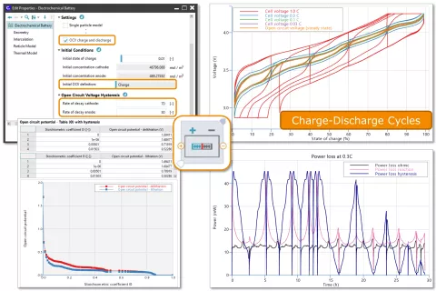
For the electrochemical pseudo-2D model (P2D) for lithium-ion cells, it is essential to be able to take into account material properties such as a characteristic hysteresis of the Open Circuit Potential (OCV) curves. New in this version of AVL CRUISE™ M is the ability to consider OCV hysteresis using two separate OCV curves.CRUISE M's material database also supports hysteresis modeling by providing the ability to process separate OCV curves for lithiation and delithiation.
Electrochemical Battery – Particle Size Distribution
Electrochemical pseudo-2D that considers only one representative particle revealed significant deviations compared to measured discharge capacities, especially at high load conditions. To overcome this deficiency, this version of CRUISE M extends the possibility to consider the impact of particle size distribution (PSD) in its material database and as part of the Electrochemical battery component itself. In the material database, you can now choose between the input of log-normal or normal distributions or opt for a table-based specification.
In addition to phenomenological modeling of the open circuit potential hysteresis and particle size distribution, CRUISE M now includes detailed simulation of variable solid state diffusion. With these three new functionalities, it is well equipped for modeling LFP or Si-dominated electrodes.
Electrochemical Battery – Electrode Balancing Wizard
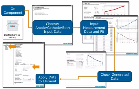
A new electrode balancing wizard has been added to the existing wizard collection. It complements the existing EIS wizard to facilitate the efficient parameterization of accurate P2D models. The wizard supports in parameterizing fundamental Electroc-Chemical Battery (ECB) model parameters, which describe electrode capacities and open circuit voltage with the help of data from half-cell and three-cell electrode measurements.
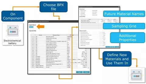
Electrochemical Battery – BPX (Battery Parameter eXchange ) Import
An open standard for physics-based lithium-ion battery models has been launched by The Faraday Institution back in 2022 (see The Faraday Institution, bpxstandard.com). The Battery Parameter eXchange (BPX) standard covers parameters which can be used for Doyle-Fuller-Newman (DFN) and Single Particle Models (SPM) and includes key battery parameters for anode, cathode, electrolyte and separator materials.
This version of CRUISE M provides a BPX import wizard that enables users to read in human readable JSON files to parameterize the electrochemical battery models. The parameters are transferred to the CRUISE M and AVL FIRE™ M material database and stored as new, user-specific materials.
Engineers working on battery models using PyBaMM now can go beyond the battery cell, into system simulation.
Cylindrical Battery Module Component
The cylindrical battery module in CRUISE M has received enhancements to model cooling channels in even more detail. With this version it is possible to define thermal interface layers positioned between the battery cells and the cooling channels.
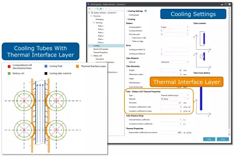
CRUISE M already offer the possibility to evaluate and assess the heat propagation between neighboring cells during a thermal runaway event for pouch and prismatic cells. This version extends this functionality to the cylindrical module component. It also allows considering thermal propagation between neighboring cylindrical cells via the potting material.
Equivalent Circuit Model (ECM) Battery – Full Pulse Fitting
The fitting accuracy provided by the battery parameterization wizard is raised to a new level considering voltage responses during the current pulse.
Now it is possible to choose between individually fit data from discharge or charge pulses or work with a combination of both. The new option “full pulse fit” allows fitting both voltages from pulse and relaxation phases. In this two-step approach after the initial relaxation voltage is fitted in the second step, the generated parameters are refined by fitting pulse voltages.
Battery Thermal Analysis in AVL CRUISE™ M
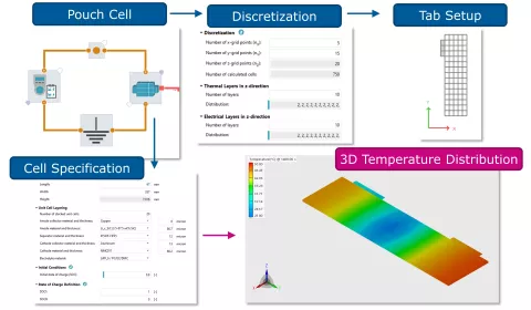
This version of CRUISE M introduces a new pouch cell component that offers a scope known from CFD codes while sticking to the ease-of-use known from system-level simulation.
The electrochemical battery component in CRUISE M is multi-physical and multi-dimensional. Detailed electrochemistry is embedded in 2D models for current distribution in collector plates and 3D thermal model. The pouch cell component supports investigations on cell arrangement and tab positioning without the need of CAD models.
Battery Thermal Analysis in AVL FIRE™ M
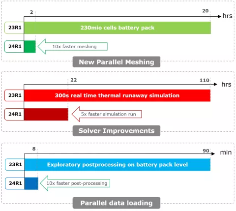
FIRE M has received its biggest update in years. These updates are particularly aimed at large and complex geometries, such as those found in battery packs. And it includes all parts of the workflow: new preprocessing flexibility, simulation speed and capabilities as well as postprocessing speed.
This also applies to the FIRE M battery thermal runaway workflow, which has been completely overhauled in its basic structure and has received significant updates and new features that increase the usability and adjustability for the user.
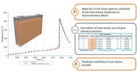
Battery Thermal Runaway – Solid Body Chemistry
Heat release within the battery cell can now be modelled in FIRE M using the solid body chemistry feature. The user can provide a reaction mechanism to predictively model the battery heat release due to decomposition, melting and reaction of components in the battery (e.g.: cathode, anode, SEI …). These mechanisms make use of detailed chemistry calculations of battery components as representative species (meaning e.g. anode is a species) and their respective heat release in a reaction mechanism.
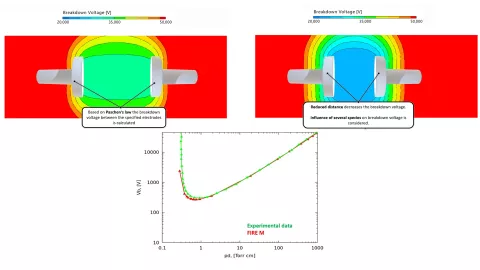
Battery Thermal Runaway – Breakdown Voltage
The venting gas itself can lower the breakdown voltage between two current carrying parts and therefore increase the risk of arcing. With the new release of FIRE M it is possible to calculate the breakdown voltage with respect to the selected venting gas species.
SOxC System Generator
The setup of solid oxide stack and balance of plant (BOP) system models can be a demanding task, calling for expertise in the required stack configuration, the media supply components, their sizes, arrangement, and controls to run transient simulations.
The present release of AVL CRUISE™ M facilitates the setup of such models with an SOxC System Generator that, in its simplest approach, requires nothing more than two single stack characteristics: the active cell area and the number of cells in the stack. In an optional input branch, you can configure the details of the reaction chemistry taking place in the stack. With that configuration, you can efficiently create a simplified system model, sufficient to operate the stack.
Optionally, a more detailed standard BOP system model can be generated, featuring a blower, heat exchangers and oxidation catalyst as well as controls to operate the complete system. The automatically generated model, featuring estimated component parameters, is ready to run. It offers a dedicated simulation dashboard and built-in result previews.

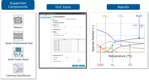
Chemical Equilibrium – Kinetic Free Species Conversion
The calculation of chemical equilibrium (CE) is a well-established method for assessing the impact of chemical reactions on species conversion, both in the gas phase and beyond.
This version of CRUISE M allows you to perform CE calculations using a new chemical equilibrium component and with the option to calculate chemical equilibria in the plenum, quasi-dimensional pipe and solid oxide stack components. When activating the CE calculation, you are guided through the configuration step for the calculation.
The entire CE calculation is performed with the help of the Cantera package, offering single-phase and multi-phase equilibria depending on the presence of non-gaseous reaction partners. The applicability of the CE approach is validated for a solid oxide fuel cell (SOFC) system model, where the kinetic conversion calculations of the fuel reformer and afterburner catalyst can optionally be substituted by CE calculations.
The CE functionality is also embedded in the SOxC wizard to consider the impact of stack internal fuel reforming reactions. A simple sandbox installation example and a real-life SOFC system demo model are ready to give you a quick start.
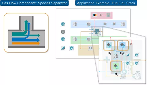
Species Separator – Custom Reaction Modeling
CRUISE M supports the modeling of chemical or electrochemical reactions involving gas species through dedicated components such as the chemical equilibrium or stack components. However, there are reaction constellations that are not fully covered by these library components.
This version of CRUISE M lifts this restriction with the introduction of a new species separator component. You can pull it from the library and connect it to plenum and quasi-dimensional Pipe components and selected transfer components in a side flow configuration. In the species separator component itself you can select which species shall exclusively be added or removed from the gas path.
When connecting the separation mass flow rate with compiled function components, you have everything at hand to model any kind of chemical reaction. There are two installation examples showing hydrogen separation from a gas stream and how to model a custom fuel cell stack. It is certainly worth looking at these models for inspiration.
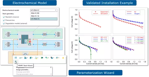
High-Temperature PEM Fuel Cell
High-temperature PEM fuel cells (HT-PEMFCs) are an interesting alternative to conventional low-temperature fuel cells. They operate at temperatures up to 200°C and are known to be less sensitive to impurities of the supplied hydrogen.
CRUISE M addresses this technology with a new HT-PEMFC stack model with its electrochemical performance tailored for high temperature applications. This includes the formulation of the Nernst equation and the calculation of ohmic and transport losses, all considering the absence of liquid water.
The model is validated with data from literature, i.e. polarization curves at different temperatures, feed gas concentrations and feed mass flow ratios. The comparison shows excellent agreement, thus confirming the model adaptions regarding e.g. the temperature dependence and scaling of the activation losses.
Model parameter identification is fully supported by the existing PEMFC stack wizard. To get a jump start on HT-PEMFCs, visit the corresponding installation examples.
Chemical PEM Fuel Cell Degradation – Speed and Robustness
CRUISE M's Chemical Fuel Cell Degradation component offers a comprehensive and powerful approach to investigate various cathode catalyst and membrane degradation phenomena. This comprises effects like carbon corrosion, platinum particle detachment and agglomeration, as well as ionomer degradation due to the formation of OH radicals out of H2O2 via a reaction with ferrous ions (Fenton's reaction).
As you might imagine, the computational demands of the reaction and transport models behind all these phenomena can significantly affect simulation time. This version of CRUISE M introduces analytical measures applied on the set of constituting equations to support numerical procedures resulting in computation speedup of 20% to 40% at unchanged accuracy.
Aging investigations covering hundreds of physical operating hours, running the degradation model in a closed loop with a PEMFC stack model, can thus be handled in an efficient manner.
PEM Fuel Cell Stack Wizard – Raised Flexibility
This version of CRUISE M offers an upgraded PEM fuel cell stack wizard, enabling you to start the parameterization process from an existing PEMFC Stack component and to store all reference data in case you would like to revisit, modify, and rerun the parameterization procedure. This new approach implicitly offers one additional important enhancement. All initially given stack model settings and parameters, including the material properties, are taken over by the wizard and considered in the parameter optimization process. Generating nothing else than a running PEMFC stack model, of course, remains supported.
PEM and Solid Oxide Fuel Cell System – Channels for Monitoring and Control
For efficiently operating CRUISE M's PEM and solid oxide fuel cell models in HiL environments, this version of CRUISE M offers a much broader set of channels for system monitoring. This comprises e.g. channels for stack pressure drop, dew point temperature, specific heat and isentropic exponents in plenum and gas node components, minimum and maximum channel mass flows, Reynolds number and dynamic viscosity in quasi-dimensional pipe components, plenum mass, and several others.
The new channels not only expand the monitoring scope of fuel cell systems but also facilitate the implementation of control strategies in compiled function components.
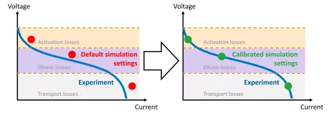
Automatic Calibration of Fuel Cell and Electrolyzer Stack Models
In this version of AVL FIRE™ M the multiphysics-based fuel cell and electrolyzer stack models can now be automatically calibrated based on measured polarization curves. For each region of the polarization curve (activation, ohmic, transport), a specific set of model parameters is efficiently optimized resulting in a unified stack model parameter set. With the unified set of model parameter values the entire ensemble of measured polarization curves is matched with high accuracy and additionally offers extrapolation capabilities even beyond the original parameter space covered by the measurements
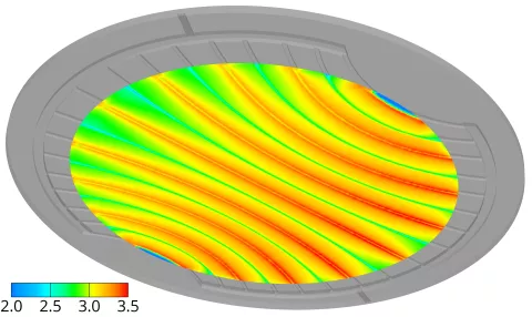
Mechanical Membrane Degradation Model
With this release of FIRE M we introduce a model specifically designed to address the mechanical degradation of PEM fuel cell membranes. The model accounts for various factors affecting membrane durability, with a focus on clamping pressure, changes in water content, and temperature.
As the PEM fuel cell operates, variations in water content and temperature induce swelling and shrinking of the membrane. These changes create tension and deformation energy, impacting its overall integrity. Based on the Eyring model, originally developed for viscous materials, we extended this model by incorporating thermal effects and creep behavior specific to PEM fuel cell membranes.
Refined Liquid and Dissolved Water Treatment
A set of model refinements are now available with this release of FIRE M for the treatment of liquid and dissolved water in the catalyst layer of low temperature fuel cells, electrolyzers and hydrogen compressors.
For low temperature PEM fuel cells and PEM hydrogen compressors an individual transfer coefficient is used for the mass transfer between the liquid phase and the dissolved phase.
For PEM and AEM electrolyzers, additionally an individual equilibrium water content is used for the liquid phase which usually depends on the temperature. The separate consideration of the liquid phase in the water mass transfer to and from the dissolved phase yields further improved results for cases in which liquid water plays an important role.
The main effects of the model refinements can be observed in electrolyzers, where the mass transfer from the liquid phase to the dissolved phase is treated more realistically, thus leading to increased accuracy in simulated cell performance.
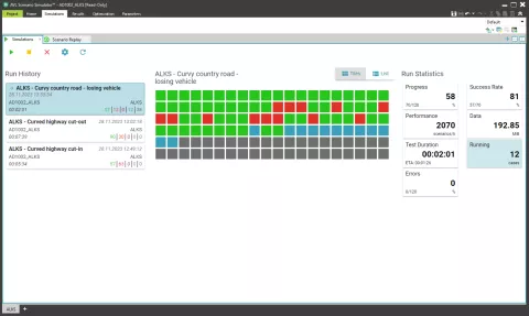
Introducing the New Freemium AVL Scenario Simulator™
AVL Scenario Simulator™ is the cost-optimized solution for fully automated, large-scale ADAS/AD testing based on the ASAM OpenSCENARIO® XML standard. Continuously integrate and test your planning and controls stacks in our flexible and open simulation platform for faster feedback loops and higher test coverage.
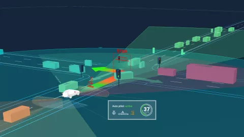
Build the optimal virtual prototype for each test purpose. Open interfaces offer maximum flexibility with easy integration of your ADAS/AD software and other simulation models or tools.
High-performance object-based sensor models are the missing piece that enables scalable closed-loop testing of planning and controls without resource-intensive physical sensor simulation. The object-based sensor models natively support the ASAM OSI®(Open Simulation Interface) standard adding geometrical, phenomenological and / or statistical effects to the ideal ground truth. Simulate virtual prototypes with more than 40 sensors faster than real-time and highly parallelized. As only CPUs are required to run the simulation, scaling to thousands of parallel simulations is very cost-efficient.
The freemium version of the tool can be used free of charge with all features, but for a limited number of simulations per day. You can upgrade for unlimited simulations anytime and get access to our expert support team or a seamless integration with the certified safety argumentation toolchain AVL SCENIUS™.
Stay tuned for the upcoming launch event and webinar series.
AVL Scenario Designer™ – OpenSCENARIO XML 1.3 and Support for Custom Traffic Signs
With the new release, AVL Scenario Designer™ supports creating, importing, verifying, and exporting scenarios in the newest version of the standard – OpenSCENARIO XML 1.3. Of course, users can still choose between all versions of OpenSCENARIO 1.x.
Besides many enhancements and bug fixes, a nice new feature we want to highlight is the support for custom traffic sign icons. When users import OpenDRIVE road networks with traffic signs from different countries, our tool will always show the position of the traffic signs and when hovering with the mouse, all information from the OpenDRIVE is provided. Scenario Designer currently comes with a full icon set for German traffic signs. Icon sets for any other country can now easily be added by copying to the Scenario Designer folder. Based on folder names (country code, revision) and the icon file names (type, subtype), Scenario Designer automatically detects new traffic sign icons and visualizes them in the imported OpenDRIVE map. This new feature gives full flexibility to our international users to easily improve the visualization of localized content.

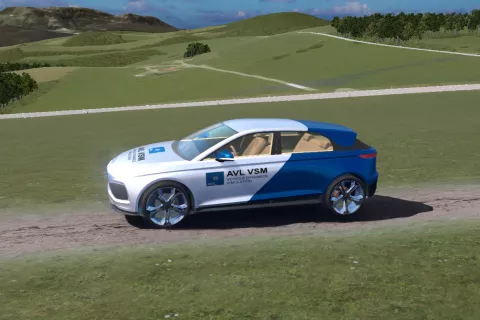
The new AVL VSM™ release extends off-road simulation to passenger cars and includes Vehicle Model Factory capabilities for commercial vehicles.
New AVL VSM™ Off-Road Simulation for Passenger Cars
The off-road performance of passenger cars from different markets is expected to improve during the coming years. This can be related to the increase of crossovers and SUV models available in the market and the usage of new technologies. Improvements that would require special and expensive hardware and controls for ICE vehicles can now be done only with new control functions for (P)HEVs and BEVs, as for many of them the hardware is already available.
Testing on off-road conditions, such as on dirt, sand, mud or snow roads is very difficult in real life, as the track conditions are constantly changing based on soil deformation and due to weather conditions. For each different test day, the road looks different, that makes the vehicle development, calibration of controls and validation challenging. To provide a reliable test condition, AVL VSM™ 2024 R1 introduces the off-road feature also for passenger cars.
This solution enables a consistent and reproduceable soil condition for off-road virtual development, calibration and testing. It included pre-defined roads, soil conditions, tires and vehicle templates that, when combined with the ready-to-use VSM powertrain options and vehicle control models leads to an efficient workflow and high simulation accuracy. The well-known real-time VSM capability also applies to the off-road topics, enabling XiL usage.
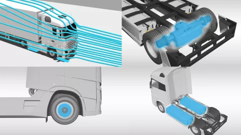
Vehicle Model Factory Includes Commercial Vehicles
VSM had the first public release of the Vehicle Model Factory during year 2021, focusing on passenger car model build-up and validation. Since then, the extension and improvements of its contribution follow the VSM road map, supporting with a simple workflow the identification of several different vehicle systems requested by the simulation community. The new VSM release extends the successful Vehicle Model Factory feature to commercial vehicles.
Setting up a complete vehicle model from scratch and validating before initial development and testing activities start is no longer a cost and time-consuming task. This is the first public release that includes artificial intelligence for commercial vehicles. Parameters related to driving losses, electric drive units, battery, or internal combustion engine, steering and brakes are identified automatically from road / proving ground measurement data.
Existing measurements can be reused to automatically build and validate systems or the entire vehicle, or new tests can be performed with easy-to-use data acquisition setups. E.g. using systems compatible with SAE1939 standards or a specific DBC file related to the vehicle under test. GPS data can also be imported, meaning that a lot of alternatives are possible, including the usage of permanent vehicle loggers commonly integrated.
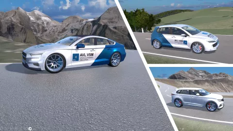
Vehicle Template Generator Is Released as Part of AVL VSM™
During initial development phases and in any situation when vehicle input or measurement data is not available, the model build-up process can rely on existing VSM vehicle templates as a start point for development, optimization, and testing. When modifications of these templates are necessary, the user experience plays an important role and is normally applied (considering that Vehicle Model Factory can’t be used due to lack of measurement data).
Some users are not experienced in all vehicle systems (e.g. chassis, powertrain, battery …) due to the complexity increase over the years. In order to provide a brand new solution that is fully integrated with VSM, we have developed the Vehicle Template Generator. Starting from defining expected KPIs (physical results, e.g. 0-100 kph time) and boundary conditions, an artificial intelligence model optimizes the vehicle parameters to match the expected results.
This is not a standalone method, as it can be combined with input data that is already available or using partial measurements in Vehicle Model Factory and vice-versa, the new Vehicle Template Generator can be used as a complement of Vehicle Model Factory, meaning when measurements are missing, it can be applied for those specific missing areas. With this, we set the most efficient methods for creating and validating virtual vehicle models.
AVL VSM™ is also available as part of AVL vSUITE™
The VSM 2024 R1 (including add-ons) is also part of the vSUITE 2024 R1, empowering vehicle system simulation and optimization with the unique all-in-one solution.

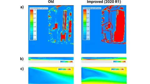
Resolving Thin Embedded Bodies Without Using the “Shell” Option
By setting the user defined parameter EMB_KEEP_SHELLS to “1”, the embedded body geometries are artificially made thicker where they otherwise would not be resolved by the CFD mesh. This means that there is at least one fully solid cell at all embedded body surfaces. As illustrated in Figure 1, the new treatment substantially improves the resolution of thin parts and consequently the predicted airflow field.
Note: If the "shell" option is activated for a body, all cells intersected by the embedded body surface are set to "full solid" anyway.
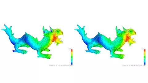
Improved Interpolation of 3D Results on Embedded Body Surfaces
When using embedded bodies, the user defined parameter "EMB_3DRES_SURFACE_NODE_VALUES" can be set to "1" in order to get 3D results for certain quantities directly on the surface mesh of the bodies. This is done in the solver by interpolating values at the surface mesh nodes from the surrounding mixed CFD mesh cells at the boundary of the surface. Mixed cells are those with a solid volume fraction larger than zero and less than one.
However, there was a potential problem that body surface nodes didn't get an interpolated value when no surface element containing the nodes was intersected by a mixed cell. This typically happened with fine body surface meshes and coarse CFD meshes as illustrated in Figure 2 (left). This has been fixed by interpolating values at such nodes from surrounding surface nodes in a second interpolation step. The figures below show the difference: on the left the old interpolation with some blue spots at the tips of the horns, tail and heels, where interpolation failed, and on the right the new interpolation, which removes these spots.
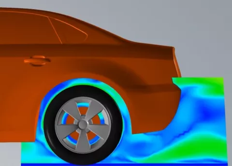
Efficient Export of the Selection-Based 3D Transient Airflow for PreonLab
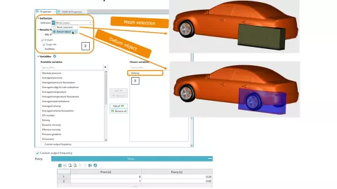
The 3D result output restricted to cell selections can be defined by right-clicking on “3D Results” in the element pane and selecting ”New 3D Result” or “select + icon” next to “3D Results”. This output is written independently of the standard 3D outputs into separate subfolders in the results/sel folder.
The selection can be specified either as mesh selection or datum object. In addition, a Custom output frequency can be activated (in this case the output frequency of the global 3D results is overwritten for this selection). If “Custom Output Frequency” is activated, the standard output may be switched off if output is desired for the specific selections only. This enables the highly efficient generation of steady or transient airflow data (written out in Ensight single file format) needed for PreonLab simulations.
Stay tuned
Don't miss the Simulation blog series. Sign up today and stay informed!
Stay tuned for the Simulation Blog
Subscribe and don‘t miss new posts.